Table of Contents

This article will discuss the relationship between price change and customer retention.
If I raise the price, will customers leave?
The biggest challenge that leaders face is understanding how to think about price optimization and customer retention with the right framework.
For example, many leaders focus on the churn metric as a proxy for customer retention. The problem with this is that churn doesn’t tell us anything about how long our customers subscribe for. After all, as some in the industry have pointed out, churn relates more to the age of our subscriptions than to the persistence of our subscribers.
In this article (this is part one of our Price Optimization series), we will discuss the relationship between price change and customer retention, as well as the best metrics and methods for measurement.
Does my new price make customers unsubscribe sooner?
Let’s consider the price example from our series introduction. Suppose we quadrupled our price, gained some new customers, and our MRR was looking good. Do we know the customers will stay just as long as they used to?
What if the higher price makes our service more noticeable in their budget, causing them to drop out sooner? Will they decide after a few months that our service is not worth it? What if we raise our prices and they don’t care?
We need an accurate way to measure our customer’s subscription lengths in order to answer these questions.
BE HONEST
How well do you know your business?
Get deep insights into churn, LTV, MRR and more to grow your business
Beware: Avoid bad metrics to measure customer retention
Typically we are told to use metrics like churn as a proxy for customer retention. These metrics will mislead us. First, let’s tackle why churn isn’t a useful metric.
Take a look at this distribution plot of known subscription lengths from an actual SaaS sample below. Next to the subscription lengths graph, we have the implied survival curve as a function of time (it shows the probability of a subscription surviving up to that time).

Notice the long tail in the distribution plot on the left. The plot has a mix of mostly short subscription lengths and a few long ones.
Now, suppose we consider the population from the graph on the left as a distinct cohort of subscribers, and they all start simultaneously. Imagine measuring their churn over time. After the bulk of customers churn out initially, the remaining customers in the long tail are the only ones remaining. This means the churn rate would decrease over time.
We can also see this in the decreasing trend in survival rates on the right. The probability curve for survival stops decreasing as fast when subscriptions get longer. Indicating the remaining customers are less likely to cancel.
This shows us that, in reality, the churn rate is not constant. As this cohort progressed over time, we saw less and less churn. The longer a subscriber subscribes for, the less likely they are to churn. The churn metric is blind to this. People assume it measures retention when in reality, all it tells us is how young or old the subscriptions are.
The churn metric won’t help us with price optimization. Let’s abandon the churn metric and look for something else!
If we can’t use churn, can we use the average subscription lengths?
We might think a good alternative to the churn metric is using the average subscription lengths. While this is partly true, chances are we are calculating it wrong.
When we simply take the average subscription lengths in our data, we aren’t actually approaching the true average. We are actually doing what we call the naive average subscription length.
Let’s think this through:

If we want to compare subscription lengths, then we should collect all the subscription lengths we have for each price, and compare their respective averages. Then we can tell if there is a difference, right?
Nope. That would be a huge mistake. When we do this, we bias our estimate against longer subscriptions. The long-lasting subscribers are more likely to be still subscribing.
These kinds of observations, where subscribers aren’t finished yet, are called censored data. We know when they began, and we know their subscriptions survived until the present. But we don’t know when they will cancel. That part is censored.
The naive average subscription length ignores these censored customers, but they are the most valuable subscribers, and their contribution is critical for us to understand our customer retention.
So both churn and naive averages are the wrong metrics to use. What options do we have for measuring customer retention?
Time for some statistics!
Since we don’t know how long the censored subscriptions will last, we need to make an educated guess. That’s where statistics comes in. We draw from a field of statistics that deals with time-to-event data, commonly known as Survival Analysis.
Instead of using naive averages in our subscription lengths dataset, we will use the data we have to build a survival model.
It is a model that attempts to describe all the possible subscription lengths and assigns a probability to each. It treats our data as a small subset of a much larger distribution of subscription lengths.
If we use the model, we can extrapolate beyond our dataset, to define the overall pattern of subscription lengths, and get accurate estimates of its features, to answer questions like “what is the average subscription length.” The correct subscription length average to use is the average subscription length seen in that model. How does this work?
First, we need to choose the distribution we will build our model with. Time-to-event data tend to follow a series of probability distributions called the exponential family. These probability distributions neatly model time-to-event processes in nature. The great thing about these is that they assign a likelihood that the subscription could reach any given length for both censored and uncensored data.
We seamlessly plug in censored and uncensored data to get likelihood estimates for each subscription length. Then we use those likelihood estimates to choose the parameters for our model, in a process called Maximum Likelihood Estimation.
We choose the parameters that maximize the likelihood of seeing the observations from our original real dataset. This ensures that our model closely fits our data.
For now, we are going to use a flexible member of the exponential family: the Weibull distribution. Other distributions may be a closer fit to our data, but we will go with this one for the sake of simplicity.
The Weibull distribution is flexible because it can handle increasing and decreasing cancelation rates as a function of time. You don’t need to understand this equation or remember it, but for those who are curious about how this works, here is the Weibull probability density function:

The shape parameter denoted alpha () defines increasing or decreasing rates of survival. The scale parameter denoted sigma (σ) determines the spread, which dials the mean subscription length.
From this, we can derive a function for the probability of surviving at least a given duration, called the Survival function S(t).
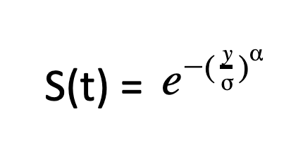
The survival function gives the likelihood of survival of censored data because, in censored data, all we know is that the subscription lasted up to a certain point of time, and that it will end at some time beyond that.
Note that the survival function also depends on both the shape and scale parameters. This allows us to use censored observations along with the uncensored ones to find optimal values for shape () and scale (α) to get the weibull distribution that is the closest fit to your data.
After we fit a model like this to the data, we can take the mean of the distribution as our estimate for average customer retention.
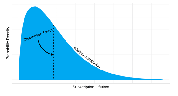
Below is an example of a Weibull distribution. This is just an example distribution to illustrate what it could look like. Moving forward we can play with the subscription price, sign up rates and customer retention to model our data:
Now let’s compare using the Weibull distribution to estimate subscription lengths with the naive average, and see the difference.
The Naïve estimate for subscription lengths is very bad
To show how much better it is to model your subscriptions with Weibull, let’s illustrate with a simulated example.
Let’s imagine 60 subscriptions following the Weibull distribution, and censor about half of them. To make things harder and closer to reality, let’s censor them early, mostly below the actual mean subscription length. We’ll compare the naive average to the estimate from a survival model assuming the Weibull distribution.
For speed, we’ll use a frequentist method for estimating the parameters with the Survival library in R.
Let’s repeat this 100,000 times and compare the results on a density plot:
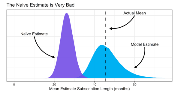
See? The naïve estimate is terrible. It underestimates the actual average subscription length all the time.
The Weibull estimate, on the other hand, tends to hit the target. Consider the challenges here: most of the data is of short duration and highly censored.
Nevertheless, the model does a great job and wins. So how can we use this in a price optimization scheme?
The next section will show two applications of the Weibull distribution.
Using Survival Analysis: The Weibull model correctly predicts subscription lengths in two scenarios
Let’s begin with a fundamental question. If we make a price change, are the subscription durations different?
What if we raise our price, collect data, and want to compare subscription durations between two price points?
Here are two examples to test using the Weibull distribution to model subscription lengths on simulated data.
Since it’s a simulated example, we already know the truth, and we can test if our method can detect it.
Scenario 1: Higher price makes subscribers cancel sooner
Let’s simulate a dataset that follows this story: say we offer a service at a low price, $20/month, and get 60 customers. We provide the same plan but raise it 80% to $36/month and get another 60 customers.
In reality, we know that many factors can affect revenue, like sign-up rates, time, marketing, and so on. But for this example, we are going to assume that these don’t affect revenue, so we can focus on understanding the relationship between price, customer retention, and revenue.
In this story, let’s assume that customers don’t like the higher price and cancel their subscriptions sooner, enough to neutralize any revenue gains.
To summarize:
- We created a data set where there are two prices being offered.
- One price is $20/month and there are 60 signups.
- Another price is $36/month and there are 60 signups.
- The customer retention is affected by price.
- We gave a longer customer retention to the lower price.
- We gave a shorter customer retention to the higher price.
- We designed it so that the LTV per customer (regardless of their signup price) is constant.
- Half the dataset is censored.
Because we’re “playing God” in this data set, all the data points in our simulated data set follow the above conditions.
So, what we will do is feed the Weibull model these simulated data points. Half of the data we feed to the Weibull model is censored. Then we will use the Weibull model to predict the customer retention based on a given subscription price.
In other words, we will let the Weibull model learn from our simulated and censored data set. Then we can plug in a subscription price, and the Weibull model will predict the subscription length for us.
This time, we fit a Weibull model using a Bayesian framework with the brms package in R, so we can visualize the marginal effects easily. We’ll add the price plan as a predictor for comparison. After we train the model, we’ll display the results on a marginal effects plot to show what the model thinks the average subscription lengths are for each plan. See the results below: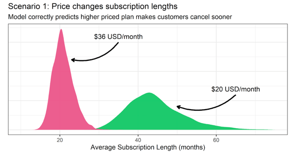
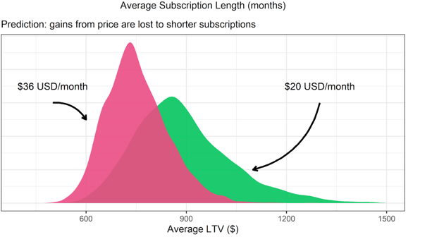
Look at that! In the top plot, we see density plots for the average subscription length for each price point estimated by the model. These are the relative probabilities assigned by the model for the estimates. The higher the peak, the more likely the model thinks the estimate is.
Notice that there is minimal overlap between the subscription lengths. We can interpret the lack of overlap as the model assigning very little probability that the average subscription lengths are the same between price points.
In other words, the model is very confident that the subscription lengths are different between plans, and that customers drop out sooner in the more expensive plan. But what does that mean for our revenue?
We get the implied revenue by multiplying the predicted durations by the respective monthly prices of each plan. This gives us an estimate of the expected lifetime value for a customer.
It shows a lot of overlap between predictions. More overlapped than not. This means that the model isn’t sure if either plan is better concerning long-term revenue.
While the less expensive price point retains more customers, it doesn’t yield more revenue. The Weibull model accurately detects this conclusion, while other methods may not be able to.
Scenario 2: Price doesn’t affect subscription lengths
Let’s pretend there is no difference in customer retention between price plans. Can our model detect this? What are the implications for revenue? Let’s set up another fake dataset, where we know that price does not affect subscription lengths.
Half of the points in the dataset will be censored. After feeding our dataset to the Weibull model, will it be able to correctly predict the subscription lengths when given a price?
Here is a summary of this scenario:
- We created a data set where there are two prices being offered.
- One price is $20/month and there are 60 signups.
- Another price is $36/month and there are 60 signups.
- The customer retention is NOT affected by price.
- We designed it so that the LTV per customer is higher in the $36/month price.
- Half the dataset is censored.
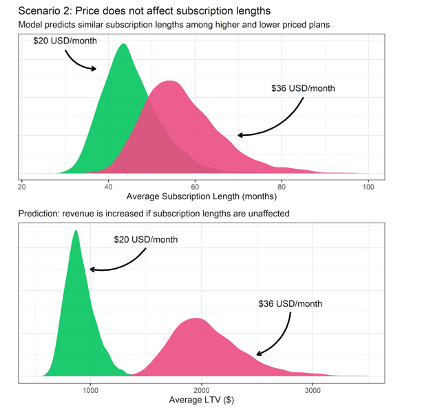
In this scenario, the model shows a lot of overlap in the expected durations between plans. This means that the model assigns a lot of probability on the subscription lengths being the same.
As a side note: the densities don’t overlap entirely because we used random samples to make our estimates, and that made them slightly different by chance.
Despite this, the estimates weren’t different enough to tell if they came from different distributions, which is correct, because we know they came from the same distribution because we simulated it that way.
When we multiply the durations by their prices, however, we see a big difference. The model is confident that the higher-priced plan is better. The higher-priced plan yields greater revenue in this scenario, because customers don’t drop out sooner.
This is a situation where correctly estimating customer retention is critical, because the model (correctly) predicts that the more expensive plan yields $2000 lifetime value on average, compared to the less expensive plan that averages $750 lifetime value.
This is all dependent on confirming that customers don’t drop out sooner, which our model also predicts correctly.
Key Learnings: Pricing and customer retention
- It’s very important to avoid churn and naive average subscription length as your metric for customer retention.
- The correct metric for measuring subscription lengths is generated through estimating the distribution that best matches the nature of our data.
- We can predict real differences in subscription lengths when the price changes using survival analysis even with highly censored data.
- Being able to model subscription lengths means we can identify a more optimal price point for our services, assuming all other factors are equal.
Beware: Correlation is not causation
It is easy to assume a causal relationship between price and duration in our simulations because we coded it that way. However, it would be a mistake to assume a causal relationship between prices and durations in the real world.
This is because many factors other than price could cause the correlation. For example, a superior competitor could enter the market shortly after a price change. Or world events like a pandemic could force your customers out of business, shortening subscriptions. Small sample size and randomness could also make an apparent correlation.
Unless we carefully construct an experiment, we can’t control for factors that confound our results. We need to be vigilant about finding any factor that could throw our predictions off.
Even if we feel very confident in our methods, we can’t possibly know all the factors that could mislead us, so we need to look at our results with a healthy dose of skepticism before we act on them.
If we do an experiment, it’s essential to control for as many potential differences between customer groups as possible if we want to be more confident in a causal relationship.
A great experiment to start with would be to compare different prices within the same cohort. Imagine an experiment similar to an A/B test, where two randomly selected customer groups are offered different prices in the same time window to reduce the chances of a spurious result. More on that in a future article!
Next Steps
You should now be thinking about experimenting with prices and estimating subscription lengths correctly to improve customer retention. Take a look at a survival analysis package in your favorite programming language and try it out.
And since we now know the metrics we need to use, how do we use them in an experiment?
Our next article will be about how to put together a price experiment, and get the right data so you can build a great model like you’ve seen in this article.
Happy experimenting! If you need help, don’t hesitate to contact support@baremetrics.com or start your 14 day free trial. We’ll show you how to understand the value you provide to your customer through price optimization.

